Top-down Non-Correcting Error Recovery in LLgen

Arthur van Deudekom
Peter Kooiman
Department of Mathematics and Computer Science
Vrije Universiteit
Amsterdam

Supervised by
dr. D. Grune
Department of Mathematics and Computer Science
Vrije Universiteit
Amsterdam

ABSTRACT

This paper describes the design and implementation of a parser generator with non-correcting error recovery based on the extended LL(1) parser generator LLgen. It describes a top-down algorithm for implementing this error recovery technique that can handle left-recursive grammars. The parser generator has been tested with several existing ACK-compilers, among which C and Modula-2. Various optimizations have been tried and are discussed in this paper.

1. Introduction

One of the trickier problems in constructing parser-generators is what to do when the input to the generated parser is not well formed. Several approaches are known, most of which are ‘correcting’, meaning that they modify the input to make it correct. However, in most cases there are several possible corrections, and often the one chosen will turn out to be the wrong one. As a result of such an incorrect choice, spurious error messages can occur. Every programmer knows from experience how the omission of a single ‘)’ can on occasion lead to pages of error messages.

A radically different approach is to just discard all the input up to and including the offending token, and start with a clean slate at the token following the offending one. [RICHTER] describes how this idea can be used to construct a non-correcting error recovery system that will never introduce spurious error messages. It is, however, possible that errors are overlooked.

In this paper we describe the incorporation of this non-correcting error recovery into LLgen, an existing LL(1) parser generator. In this introduction, we will describe in detail this non-correcting error recovery technique, give an overview of LLgen and how it handles errors, and finally describe how we have incorporated noncorrecting error recovery in LLgen.

1.1. Non-correcting syntax error recovery

Richter describes how syntax error recovery can be done without making any corrections to the input text. Richter gives three reasons why recovery without correction is desirable:

The non-correcting technique described by Richter can be summarized as follows: When a syntax-error has occurred, the input up to and including the erroneous symbol is discarded; the remainder of the input is processed by a substring parser of the input language, that is a parser that recognizes any substring of a string in the input language. When the substring parser detects a syntax error, the offending symbol is reported as another error, and the input up to and including the erroneous symbol is discarded. The process is then repeated with the remaining input, possibly finding other syntax errors, until all the input is scanned. This process yields what Richter calls a suffix analysis of an input string. Formally, given an input string x , suffix analysis produces a set of strings

and a set of symbols such that

and such that: is the longest prefix of that is a prefix of a string in the input language L, formally: there is a string such that is in L, but there is no string such that is in L;

For , is a longest substring of that is also a substring of a string in L, formally there are strings and such that is in L, but there are no strings en such that is in L;

is a substring of that is a substring of a string in L, formally: there exist and , such that is in L. Note that need not be a suffix of a string in L, if represents incomplete input is not a suffix of a string in L.

Now, the indicate points at which an error is detected. The "real" error need not be at , it can have occurred anywhere within . In his paper, Richter shows that, although this method may miss errors, it will never introduce spurious errors.

For implementing the technique, a parser that recognizes any substring of the input language is needed. If we confine ourselves to syntactical analysis, it is sufficient to construct a substring recognizer. Richter himself does not give a practical construction, but [CORMACK] describes how a LR substring parser can be constructed that handles BC-LR(1,1) grammars. In this paper, we describe the construction of a LL substring recognizer that can handle any grammar. Furthermore, our recognizer is actually a suffix-recognizer, that is, a recognizer that recognizes any suffix of a string in the input language. Our suffix recognizer has the correct-prefix property, meaning that it detects the first syntax error as early as possible in a left-to-right scan of the input. Specifically, if the input language is L and the invalid input is , it finds a string and an input symbol such that , there is a string such that is in L, and there is no string such that is in L. Because the suffix parser has this correct-prefix property, it can be used as a substring parser, because it will detect the first input symbol that is not part of a substring of the language. Because it is a suffix-recognizer, it additionally will detect incomplete input, because in that case at the end of the input the parser will not be in an accepting state.

1.2. Overview of LLgen

LLgen is an extended LL(1) parser generator. For a complete description, see [GRUNE]. LLgen can actually handle grammars that are not LL(1), because it allows the use of conflict-resolvers. In case of an LL(1) conflict, these resolvers are used to statically or dynamically decide which rule to use. As we will see later, this feature makes it necessary for the suffix-recognizer to handle grammars that are not LL(1). Semantic actions can occur anywhere in the grammar rules, and they are executed when their position is reached during parsing. A typical LLgen rule looks like

S: A { action } B

where the action is a piece of C-code, that will be executed when the parser is using the rule for S and has recognized A.

LLgen-generated parsers use correcting syntax error recovery, based on a scheme designed by Rohrich [ROEHRICH], inserting or deleting symbols at the point of error detection until correct input results. This means that actions in the parser will always be executed in an order that could also have resulted from syntactically correct input, and most importantly, once a grammar-rule is started it is guaranteed to be completed. This means that syntactic errors can never result in inconsistencies for the actions. Actions only have to deal with syntactically correct input. In a nutshell, the error recovery in LLgen-parsers works as follows: Suppose the parser is presented with correct input that breaks off before the end. The error recovery mechanism now provides a continuation path, chosen in such a way that all active rules are left as soon as possible. Effectively, the continuation path is the ‘shortest way out’. The symbols on this path are called ‘acceptable’, and end-of-file is also ‘acceptable’. Furthermore, at each point along this ‘shortest path’ there can be other terminals that would be correct; these are ‘acceptable’ as well. Now, when an error occurs, all symbols that are not acceptable are discarded, until an acceptable symbol appears in the input. The tokens on the path up to but not including the acceptable input symbol are inserted. From then on, normal parsing resumes.

1.3. Incorporation of non-correcting error recovery inLLgen

An important consideration in incorporating the non-correcting recovery in LLgen was that correct programs should suffer as little as possible in what regards compilation speed. Furthermore, the existing error recovery method has the highly desirable property that rules that are started will be finished too, thus ensuring that errors in the input text will not cause inconsistencies in the semantic actions. We have implemented the non-correcting error recovery in such a way that this property is preserved.

The way we have achieved these goals is by actually including the suffix recognizer as a ‘second recognizer’ in the generated parser. Correct programs are handled in the usual way by the parser, but if an error occurs the following happens: instead of going to the standard error recovery routine, the parser starts executing the non-correcting error handler. This process continues, reporting all errors, until the end of the input text is reached. Then, control is handed back to the standard error recovery routine. This routine will now think there is no more input, and thus start inserting tokens so as to construct a ‘shortest way out’. This ensures that all rules that were started are also finished, and no inconsistencies can occur in the semantic actions. However, this method does require some modifications to the error reporting routine. Normally, if the generated parser inserts a token, it reports this to the user, but in this case this is undesirable. The insertions only serve to maintain consistency in the semantic actions and do not signify errors, so reporting of insertions should be suppressed.

2. The LL suffix parser

In this chapter, we describe the construction of the LL suffix parser. The described parser is not restricted to LL(1) grammars, because the presence of conflict resolvers in LLgen allows for more general grammars, that may even be left-recursive. We start this chapter with a discussion of the implications of conflict resolvers, and continue with descriptions of the parser algorithm, the used data-structures, the handling of left- and right recursion, and some possible optimizations.

2.1. LLgen conflict resolvers and their implications

In grammars that are nearly but not completely LL(1), conflicts will arise in the two places where parsing decisions are made: the choice of which alternative to start (‘alternation conflicts’) and the decision to stop or continue a repeated item (‘repetition conflicts’). In order to allow LLgen to handle this type of grammar, the user can specify conflict resolvers in those places where conflicts arise. These resolvers are Boolean expressions labeling an alternative, and are evaluated when a conflict arises during parsing. If the expression evaluates to ‘true’ the labeled alternative will be taken. The Boolean expressions are expressions in C, and can consult any information available at the point they occur. However, if a syntactic error has occurred in the input, and the non-correcting error recovery starts, we can no longer rely on the conflict resolvers to guide parsing decisions. The suffix recognizer is only concerned with syntax, and will not execute any semantic actions. It recognizes suffices of correct input, but does not know or care what prefix would make the suffix a correct program; as a result, the information that conflict resolvers could use is not available, because the semantic actions that would build this information have not been executed. Therefore, the information used by the conflict resolvers is no longer reliable, and the suffix parser needs to be able to handle the underlying grammar without their help. In particular, it has to be able to handle left-recursive grammars.

2.2. The suffix parser algorithm

Our algorithm needs easy access to the grammar rules; in the description we assume there is an efficient way to access the grammar rules. In the next chapter we will describe the details of the actual implementation. For the moment, we will only consider grammars that are not left- or right-recursive. In the next section, we will discuss how the algorithm has to be adapted to handle left- and right recursion.

Suppose the grammar is G, and the input to the suffix recognizer is . Remember that parsing is always started by the ‘normal’ LLgen generated parser. It’s only after a syntactic error has occurred that the suffix recognizer will be started. The input to the suffix recognizer thus is the ‘tail’ of the input, starting at the first symbol after the position where the first syntax error was found.

Now, in order to get parsing going again, the parser scans the grammar for rules which contain symbol in the right hand side:

where and represent a string of terminals and non-terminals, possible empty. Now, for each of these rules found, and for any string ... that can be generated by it holds that ... is a substring of some string in L. This can be shown as follows, supposing that the start symbol is S and S A :

S A ...

Of course, there may very well be more than one such string .. , and one of these strings can be empty as well, if can produce empty. Now, in what we will call the predicting phase the algorithm will produce all possible symbols . Then, in what we will call the accepting phase these symbols are matched against the input, and those not matching are discarded. Then, entering the next predicting phase, the algorithm will produce all symbols , and match them against the next input symbol in the subsequent accepting phase, etc. In case one of the strings ... is empty, or the end of one of the strings is reached, some way to continue is needed; we will discuss this later. First let’s see how the algorithm produces the strings ... .

For each rule in the grammar of the form

with each a terminal or nonterminal, a prediction graph is created that looks like this:

The bottom element of these prediction graphs is an end-marker containing the left-hand side of the rule used. All these graphs have on top, and this is matched against the in the input in the accepting phase that follows, removing the from the graph. If the prediction graph is now empty, we have to find a way to continue; this case is treated later. First we will consider what to do if the prediction graph is not empty. There are two possibilities: either is a terminal, or it is a nonterminal. If it is a terminal, we are finished for the moment; if not, the algorithm scans for rules of the form

with each a terminal or nonterminal. Now, the algorithm substitutes the top of the prediction graph with the right-hand sides of all the rules found. Because there can be more than one rule, the prediction graph can now become a DAG (Directed Acyclic Graph). Supposing there are two rules with in the LHS:

the prediction graph will now look like this:

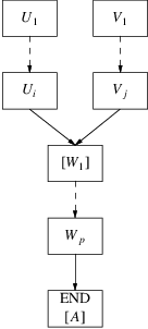
The graph element representing is left in the stack, the notation indicates it has been substituted. These substituted element will from now on be ignored by the algorithm. The elements and are now ‘on top’ of the prediction graph.

If can also produce empty, its successor in the prediction graph has to be processed as well; the algorithm walks down the graph to this successor, and there the process is repeated; if it is a terminal we are finished, else we substitute it with the right hand sides of its grammar rule. However, the element that we want to substitute now, say , cannot be marked ‘substituted’ just like that, because it can be on another path, on which it cannot be substituted yet. Therefore, a copy of element is made, it is marked , and an edge is created from to the successor of . This produces graphs like this:

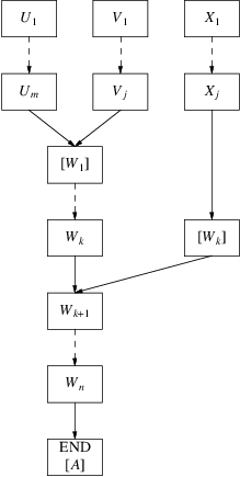
This process of substituting is repeated with all nonterminals that are now on top of the prediction graph, until there are only terminals on top of the graph. This completes the prediction phase of the algorithm, not taking into account what to do if an END marker appears on top of the graph. Now, the algorithm enters its accepting phase, in which the terminals on top are compared with the next symbol in the input. If a terminal in the graph matches the input, its element is deleted from the graph, and the substitution process will continue with its successors, in the next prediction phase. If a terminal on top of the graph does not match the input, the path it is on represents a ‘dead-end’, which does not need to be processed any further. The terminal is no longer a ‘top’, and the algorithm will not visit it again.

There is one tricky situation: consider again this graph:

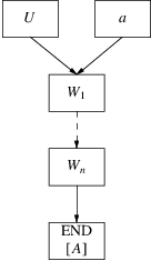
Here, the algorithm is processing in the predicting phase, and using some rule it has produced on top; there is another rule with in its LHS which has produced nonterminal on top. Now, suppose is a nonterminal that can produce empty. Now, the algorithm starts substituting , and walks down . What we definitely do not want is the algorithm to start substituting again, because then we would loop forever. Therefore, if the algorithm starts processing element it should make it before it does anything else. On entering the element for the second time in the prediction phase , it sees that it is already substituted, so there is nothing to do. It then just walks to the successor of and starts substituting it. This is correct, since the fact that the algorithm enters an element for the second time in a prediction phase means that the element indirectly can produce the empty string, and thus its successor must be substituted as well in the prediction phase.

It is easy to see that the substitution process will stop: the algorithm can only loop if it starts processing an element for the second time in a prediction phase, or if the processing of an element eventually yields a graph with that same element on top. The first case cannot occur because the algorithm marks elements it is processing as ‘substituted’ before it does anything else, meaning that those elements will not be processed again; the second case can only occur if the grammar is left-recursive, which we assumed it was not.

Now we will discuss what has to be done if an END marker appears as top of the prediction graph. When this happens, it means that starting from some rule

the algorithm has produced a leftmost-derivation of a string starting from , or that can produce empty and the string so far is just . The next step is to assume that the have recognized A and that that some string produced by is part of the prefix that makes the suffix we are recognizing a correct string in L. Remember that in the END marker we kept record of the LHS of the rule that has started the graph, and we will now use this LHS to continue recognizing. What the algorithm does is scan for all rules of the form:

with and possibly empty strings of terminals and nonterminals. The algorithm now starts a new component in the prediction graph, and if is ... it looks like this:

Note that the END marker now contains B, because we have started to match a rule for B. If the in the rule for B was empty, this just produces and END marker with B in it; in this case, the process is just repeated with all rules of the form:

etc, until we have a prediction graph with a nonterminal or terminal on top. Now, the substitution algorithm is again applied over all nonterminals on top, until every top contains a terminal. It is possible that during substitution again an END marker will turn up; if this happens we again scan for rules to continue with etc. This ‘continuation algorithm’ can only loop if, when trying to build a new prediction graph for matched symbol A, it produces an empty graph with again matched symbol A. If this happens, the grammar was (directly or indirectly) right-recursive, and we assumed that it was not. Therefore, the algorithm will terminate. The terminals on top of the new graph after applying this ‘continuation’ algorithm are exactly those that could follow the string .. in a substring of a string in L. To see this, suppose we have ‘recognized’ the rule

and ... is the string produced from by the algorithm. Now, using rule:

and supposing that S B we get

and thus any string produced by a derivation starting from can come right after ... in a substring of some string in L. The algorithm will proceed to generate all these strings starting from . If produces empty, the above is just repeated. Because in the ‘continuation’ part all possible rules are considered, the whole algorithm will recognize all substrings of any string in L. In order to determine if we have actually recognized a suffix of some string in L, we need to remember if within a predicting phase the ‘continuation’ part of the algorithm has been run on an END marker containing the start-symbol S; if this is the case, then the input seen until now is a suffix of some string in L. Formally, it means that there is a derivation starting from start symbol such that if the input seen until now is .. , then:

where can be empty, is not empty.

2.3. The prediction graph data structure

The graphs that are produced by the suffix recognizer may grow extremely large; to facilitate an efficient implementation we have devised a way of keeping the size of the data structure under control, in a way that is very similar to the way described in [TOMITA].

The basic idea is, that in a prediction phase of the algorithm, it is not necessary to explicitly substitute each nonterminal every time it turns up as a ‘top’; it is sufficient to do it once, because the second substitution will produce exactly the same subgraph starting at the substituted nonterminal. Here is an example:

Here, in the left component of the graph, nonterminal B has been substituted. Now, in the same prediction phase, the algorithm again runs into B, now in the right component. There is no need to compute again what the substitution will produce, it is exactly the part on top of B in the left component. Therefore, all that is needed is:

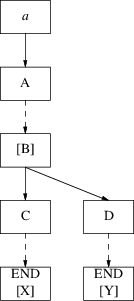
So, when, in a prediction phase of the algorithm, a nonterminal is substituted, the nonterminal is placed on a list, together with a pointer to the substituted nonterminal. If in the same prediction phase a nonterminal that is on the list becomes a top, all we need to do is place an edge between the already substituted one and the successor of the top we are currently processing. When a prediction phase is finished, the list is cleared. There is one catch: if we consider again the last picture, note that if nonterminal B can (directly or indirectly) produce empty, it is also necessary to substitute D. However, it is not difficult to determine if a nonterminal can produce empty. LLgen already computes this information for each nonterminal.

Without this ‘joining together’ of graph components, each element in the graph has exactly one successor, except the END marker, which has none. Now that components get joined as described, an element can have any number of successors. The recognizer algorithm now has to consider all successors of a graph element instead of one.

2.4. Handling right recursion

The only problem right-recursive grammars cause in the algorithm is in the ‘continuation’ part; they can cause this part of the algorithm to loop forever. As an example, consider:

Now suppose the ‘substitution’ part of the algorithm has turned up an END marker with nonterminal A in it. The continuation algorithm will now produce:

etc. etc. However, a slight modification to the algorithm suffices to eliminate this problem; within each prediction phase of the algorithm, we simply maintain a list of nonterminals that have turned up in an END marker. As soon as an END marker turns up whose nonterminal is already in the list, we stop the ‘continuation’ algorithm; the part of the graph that would be produced by it already has been generated by an earlier invocation of the algorithm in the same prediction phase. At the end of a prediction phase, when all heads are terminals, we clear the list. This way, no looping can occur; even if the right recursion is indirect, for instance if in the above example the rule for A had been

where can produce empty, the algorithm still works; the substitution of will yield an END marker on top, and when trying to find a continuation for LHS A the algorithm notices A is already on the list.

2.5. Handling left recursion

Left-recursion is, unfortunately, a much tougher problem than right-recursion. The result of left-recursive grammar rules is that the substitution algorithm never stops, because it can keep on building the graph with the same set of rules without ever turning up a terminal. One course of action would be to pre-process the grammar rules to eliminate left-recursion; there are algorithms that eliminate direct and indirect left-recursion. However, we have taken another course; by allowing the produced graphs to contain loops, we can handle left recursion without any modifications to the grammar. As soon as we come to the point that we want to substitute a nonterminal which was already substituted earlier on the same path and in the same prediction phase, we can make a link from the ‘older’ nonterminal to the successor of the ‘new’ nonterminal. In this way we have constructed a loop in the graph. As an example, suppose we have the following rules:

D: A

A: B a

B: A | x

Suppose also that we have nonterminal ‘D’ on top of a stack. We now start substituting ‘D’:

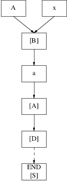
We now have an ‘A’ on top of of the stack which was already substituted on the same path and also in the same prediction phase. To avoid never ending substitution we make a loop as follows:

The dashed box with ‘A’ in it means that it can be deleted, because there is already an occurrence of it in the loop.

The most beautiful result of loops in graphs is that the original parsing algorithm needs only one minor change. When the algorithm visits an element which has more than one outgoing edge the algorithm starts tracking down both paths, just like before, only now there may be one or more backedges among these edges, but the algorithm needs not to be aware of this fact. The only difficulty with loops is that the algorithm might go into a loop; it continues searching for terminals but it might happen that there are no valid terminals in the loop. The solution to this problem is not very difficult; just set a flag at all elements we visit. When we reach an element which has this flag turned on, we don’t have to search any further. At the end of the prediction phase, when we have found all possible new heads, all flags are cleared. Even if there are no loops in the prediction graph, setting flags may be used as an optimization: it is possible that two paths come together at one point. In that situation it is useless to scan for the second time the part of the graph which both paths have in common.

2.6. Some optimizations using reference counts

As explained in section 2.2, it is sometimes necessary to copy a prediction graph element before substituting it. In order to determine if a certain element has to be copied, it is convenient to maintain a reference count in each graph element. This reference count keeps track of the number of edges that enter an element. Now, when we want to substitute an element with reference count not 0, we need to copy it, because there is another path in the prediction graph that contains the element we want to substitute, and on this other path the element cannot be substituted yet.

Maintaining reference counts also enables us to perform another optimization: remember that if, in a prediction phase, a terminal is predicted that does not match the current inputsymbol, we from then on just ignore the path in the graph starting at the terminal. However, we can safely delete the terminal from the graph; furthermore, all its successors in the prediction graph that have reference count 0 can be deleted as well, as can their successors with reference count 0, etc. This way, we delete from the prediction graph most elements that are no longer accessible, but not all of them; as will be explained in the next section, loops in the prediction graph can cause problems.

2.7. The algorithm to delete inaccessible loops

Deleting graph elements which are no longer reachable is not as easy as it looks when there are loops in the graph, introduced by the extension to the algorithm that handles left recursive grammars. Suppose for example that we have a very simple loop as in the left picture below:

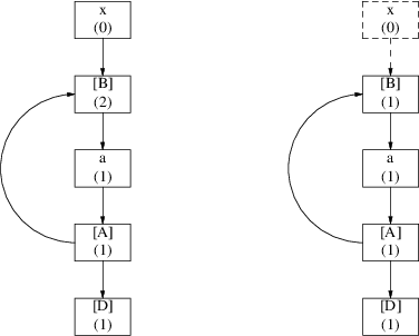
The number below each symbol indicates the reference count of that element. Suppose now that we delete ‘x’, then we have the situation depicted in the picture on the right. The loop consisting of ‘[B]’, ‘a’ and ‘[A]’ is now unreachable, so all these elements can be deallocated. The reference count of ‘[B]’ is 1, so it will not be deleted. To be precise all elements in the loop have their reference counts on 1, and consequently none of these will be deleted. But we stated earlier that all elements of the loop cannot be reached anymore and that the loop had to be deleted! In this example the reference counts of the loop elements are all 1, but in more complex situations it is also possible that some of the elements have a reference count of more than 1.

To solve this problem we present an algorithm, devised by E. Wattel, that determines whether a loop can be deleted or not. The algorithm consists of two parts. The first part of the algorithm goes as follows: it presumes that all elements of the loop will indeed be deleted. Every time it deletes an element it decreases the reference count of all the successors of the element that are also member of the same loop. How the algorithm knows which elements belong to the loop and which do not will be explained later. The situation of the example above will now look like this:

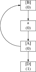
The number below each symbol indicates again the reference count after we have applied the first part of the algorithm.

The second part of the algorithm checks and restores the reference counts of all members of the loop . When it finds out that one or more reference counts are not 0, it concludes that it is still possible to enter the loop in some way, and that it cannot be deleted yet. In the other case it reports that the loop can be deleted, which is also true in our example.

We will now formally describe the first part of the algorithm that finds all directed circuits from a given vertex, and determines if the vertices on those circuits can be deleted. The algorithm works on prediction-graphs in which every edge that is in a circuit is marked. Note that a marked edge may be in more than one circuit. We will call this mark ‘C’. The input to the algorithm is such a prediction graph, and a start vertex, say A. The first part of the algorithm is:

It is clear that the algorithm will terminate: each edge is only traversed once, and the number of edges is finite. We will now prove some properties of this part of the algorithm.

An edge is traversed by the algorithm if and only if it is on some directed circuit ... .

The if-part is easy; if an edge connecting vertices and is on some directed circuit starting in , then there is a path ... ; let ... be a path of minimum length from to . If the length of the path from to is , then after turn of the algorithm will be on list L. To see that this is the case, suppose that is not on list L after turn ; this means that the edge entering was already marked used in a previous turn, but then there would be a shorter path from to , contradicting the assumption that the path is of minimum length. The edge is marked ‘C’, because it is in a circuit; it is marked ‘unused’, for if it were marked used, there would be a shorter path from to . So, in turn , the edge will be traversed.

On the other hand, suppose that an edge is traversed by the algorithm; we will show by induction on the number of turns the algorithm has made that is on a directed circuit .. . In the first turn, all edges from that are marked ‘C’ are traversed, and clearly, if an edge from is part of a circuit then that edge is part of a circuit from to . Now suppose that in turn an edge connecting vertices and is traversed. This means the edge is marked ‘C’, so it is part of some circuit. If there is a path from to , we can simply trace a circuit ... ... , and clearly is on a circuit from to . Now, suppose there is no path from to . We can always trace a circuit ... because the edge from to is part of a circuit; and by the induction hypothesis there is a circuit ... ... . We can now make a ‘detour’ at , yielding a circuit ... ... ... . This case is shown in the picture below. So in either case is on a circuit from to .

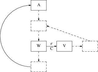
A vertex appears on list L if and only if it is on some directed circuit from to .

If a vertex is in such a circuit, there is an edge that enters it, which is part of a circuit form to ; we already showed that this edge is traversed by the algorithm, and thus the vertex will appear on list L. Conversely, if a vertex appears on list L, then an edge entering that vertex has been traversed by the algorithm; we showed that this edge is part of a circuit from to , and thus the vertex is part of a circuit from to .

When the algorithm is finished, each vertex that is part of some directed circuit from to has its reference count decreased by exactly the number of edges entering it that are part of a directed circuit from to .

Each edge that is part of some circuit from to is traversed exactly once; the reference count of the endpoint is decreased by one after an edge has been traversed. Thus, if a vertex is endpoint of such vertices, its reference count is decreased by .

If the reference count of each of the vertices visited by the algorithm is 0 after the algorithm has finised, all these vertices can be deleted; if the reference count is not zero for one or more of the visited vertices, then none of them can be deleted.

Suppose all visited vertices have reference count 0; this means that each of the vertices is only entered by edges that are on a circuit from to . Therefore, it holds that any path leading to any of the visited vertices has to start in one of the visited vertices; there is no path starting in an unvisited vertex to a visited one. Thus, all the visited vertices are unreachable. Conversely, if one of the visited vertices has reference count not zero, then there is a path from an unvisited vertex to this vertex. Because from the vertex with reference count non zero, we can get to , and from we can get to any of the other vertices, all visited vertices are reachable.

The second part of the algorithm now checks if all reference counts are zero, and if they are, it deletes all visited vertices.

2.8. Marking loop elements

One point we have omitted so far is how the edges in the prediction graph that are part of a loop get marked. Basically, a loop can be detected:

The first approach checks if a loop is constructed as soon as we join two paths in the graph, and if so, marks all edges of the loop. The other approach does not do any checking when two paths are joined together; it starts looking for loops when we want to delete an element with reference count not 0, marking all edges belonging to the loops it discovers. In practice it turns out that we very often encounter elements that we would like to delete, but that have reference count not 0, whereas the joining of paths occurs relatively infrequently. We therefore have chosen to check if a loop is created when two paths in a prediction graph are joined.

Now the question arises how to find and mark all edges of the loop. For this problem we devised also an algorithm. Because we already know that there is an edge from the element on which the new path is connected to the successor of the joined element, the algorithm only has to find a path from this last element back to the first one. This can be done by a backtracking depth first search; to find a path from one element to another we have to find a possible empty path from one of the successors of the first element to the last element. As soon as we have found a path, we can mark all the edges on the path and also the backedge as loop edges. In case that there is more than one path back to the first element it is necessary that the algorithm continues searching after it has found one path.

To avoid looping of this algorithm we have to set a flag at the elements which are on the path already. When the algorithm is backtracking it can clear the flags at the elements it is leaving.

To speed up the searching process we can set flags at the edges we have already visited but did not lead back to the first element. When the algorithm encounters such an edge it already knows that this edge is not worth searching again and can be skipped. At the end of the algorithm these flags have to be cleared again.

One might propose another optimization: as soon as we reach an edge that is already marked as a loop edge, we can stop searching for other loop edges. There is, however, a case in which this can go wrong. Imagine the following situation:

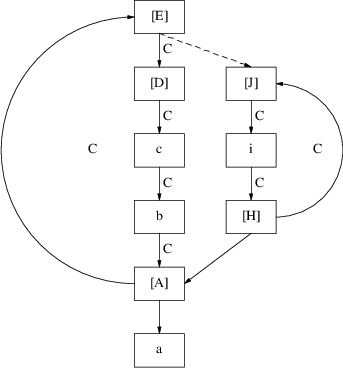
What we have here is a prediction graph with two loops; all edges that belong to a loop are again marked with an ‘C’. Note that the edge between ‘[H]’ and ‘[A]’ is not a loop edge. Suppose that ‘[J]’ is not yet completely substituted, i.e. there is another production rule for J:

The ‘E’ on top of the right path is now joined with the ‘[E]’ on the left path, which is depicted by the dashed arrow between ‘[E]’ and ‘[J]’. When we take a good look at the graph we see that the two loops are merged into one. But that is not the most important observation we have to make: not only the edge between ‘[E]’ and ‘[J]’ must be marked as a loop edge, but also the edge between ‘[H]’ and ‘[A]’! So it is not possible to stop searching for loop edges as soon as we have found an edge which was already marked as a loop edge. We have to continue until we reach the element at which we started: ‘[E]’. So the optimization proposed above is incorrect.

2.9. Optimizations using FIRST and FOLLOW sets

In the algorithm as we have described it, every nonterminal on top of the graph is substituted until only terminals remain on top; these terminals are then matched against the current input symbol. However, by using FIRST sets, we can save considerably on the number of computations necessary. Suppose one of the top elements of the graph is nonterminal A, and the current inputsymbol is . Then, it is of no use to substitute A if terminal is not in FIRST(A), because then substituting A will never produce on top of the graph. So, before substituting a nonterminal we check if the current inputsymbol is in its FIRST set; if it is not, we can declare the path the nonterminal is on a dead end, and delete it, without having to perform the actual substitution. Of course, if A can produce empty, we still have to consider its successor in the graph.

Similarly, when we have an END marker on top, with nonterminal B in it, and we consider using rule

We first check if the current inputsymbol is in FIRST(C); if this is not the case, there is no need to start a graph component with this rule, because it will never produce the next inputsymbol on top. Again, if C produces empty, we still have to evaluate the part of the rule following C.

To circumvent the problems caused in the FIRST set optimization by nonterminal that produce empty, we can also make use of FOLLOW-sets. When substituting, if we encounter a nonterminal whose FIRST set does not contain the current inputsymbol but which can produce empty, we check if the current inputsymbol is in its FOLLOW set. If it is not, there is no need to process its successor. Similarly, in case we are processing an END marker as explained above, there is no need to process the part of the rule following C if FIRST(C) does not contain the input symbol, or C produces empty but the inputsymbol is not in FOLLOW(C).

3. Test results

In this chapter, we discuss some test results that were obtained by recompiling existing ACK compilers with the modified LLgen. We tried several combinations of possible optimizations, including ‘dumb’ ones, like no optimization at all, not even deleting unreachable prediction graph elements. The incorporation of LLgen with non-correcting error recovery went smoothly; only minor modifications to the Make-files were necessary. Specifically, these modifications consisted of passing an extra flag to LLgen, and including the new generated C-file Lncor.c in the list of generated C-files. Also, the LLmessage error reporting routine had to be adapted. We successfully recompiled the C, Modula-2 and Occam compilers; in the next sections, we discuss some test results that were obtained with the Modula-2 and C compilers.

3.1. Performance

We will now present and discuss, with the aid of some diagrams, time and space measurements on the non-correcting error recovery. We have measured the effect of various optimizations. These optimizations include the first-set optimization and the follow-set optimization. We also measured the effect of leaving out the loop-deletion algorithm, regarding both time and space. We performed out measurements using C- and Modula-2-programs of three different sizes; one of approximately 750 tokens, one of appr. 5000 tokens and one of appr. 15000 tokens. We have chosen to represent the sizes of programs in the number of tokens instead of number of lines, because the number of tokens more realistically reflects the load the programs put on the error recovery mechanism. Also we give our time measurements in usertime instead of realtime, because realtime depends heavily on the load of the system, which usertime does not. Our space measurements are based on the size of the prediction graphs. Note that all files are entirely recognized by the non-correcting error recovery technique. We achieved this by putting a ‘1’ at the beginning of each file; because then each file starts with a syntax error LLgen is forced to continue with the non-correcting error recovery.

3.1.1. Time and space measurements on the effect of thefirst-set optimization

In the diagram below we show our time measurements we got from recognizing the C-programs both with and without first-set optimization.

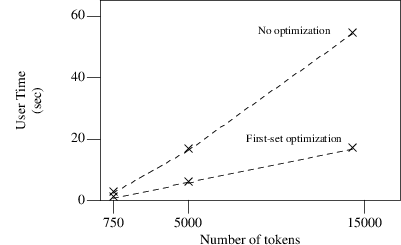
Time measurements of three C-programs with and without first-set optimization

Notice the considerable time savings we get when the first-set optimization is turned on; a factor of slightly more than 3. Obviously this is an extremely useful optimization. On the other hand we found there were no measurable time savings when using the follow-set optimization; for that reason we did not chart the result of this optimization. It seems that the time savings gained by the optimization are waisted again by the extra processing time needed. We conclude that this optimization is of little or no use when we want to save on time.

In the following picture the time measurements of three Modula-2 programs are given, again with and without first-set optimization.

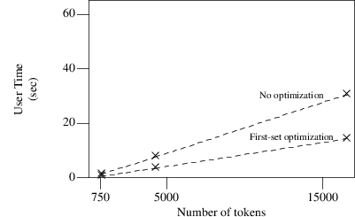
Time measurements of three Modula-2-programs with and without first-set optimization

From this picture we can conclude mainly the same as above; considerable time savings when we use the first-set optimization; the factor is somewhat less, but still more than 2. Again we have omitted the results of the follow-set optimization, for the same reason as before.

There is however one remarkable difference between the two languages: parsing C-programs needs almost twice the time as parsing programs of comparable sizes written in Modula-2. This can be explained by the fact that the C-grammar is far more complicated than that of Modula-2, and also the production rules are longer in C, so building, deleting and definitely traversing the graph will consume more time.

Now we come to the space measurements of both C- and Modula-2 programs. In the picture below we present the maximum sizes of the prediction graphs, during the recognition of the three C-programs.

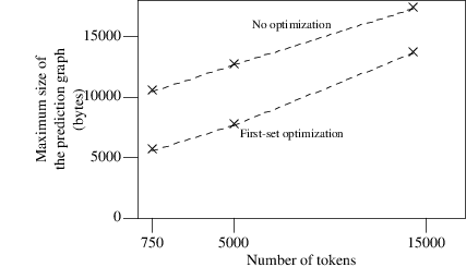
Maximum sizes of the prediction graphs when recognizing three C-programs

From this diagram we see that, although the prediction graphs are smaller when the first-set optimization is used, the space savings are not as spectacular as the time savings achieved by this optimization.

In Modula-2 the first-set optimization also causes a decrease in memory usage. The savings are less than in C, but still about 1.5 Kb. Again this can be explained by the fact that the rules of the Modula-2 grammar are shorter than that of C.

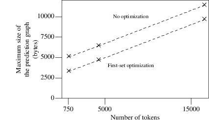
Maximum sizes of the prediction graphs when recognizing three Modula-2-programs

3.1.2. Input that is recognized in quadratic time

The measurements presented may suggest that the time required to recognize input depends linearly on the length of the input; however, this is not always the case. When there are recursive rules in the grammar, the time needed to recognize input that is produced by this rules can become proportional to the square of the input length. Consider this set of grammar rules:

When the input is ‘{aaa....’, the algorithm will produce the following prediction graphs:

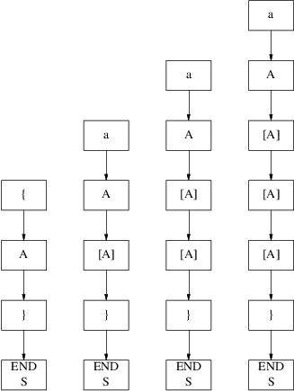
In each prediction phase, a new [A] appears on the prediction graph. However, since A also produces empty, the prediction algorithm has to traverse all the elements [A] until it finds the element ‘}’. In the first prediction phase, there is one element [A], in the second there are two, etc, so in all 1 + 2 + 3 + ... 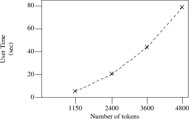+ k = elements have to be traversed if there are k prediction phases, making this proportional to the square of the input length. We constructed a parser with this simple input grammar and measured the processing time the error recovery mechanism used. In the following diagram the dashed line shows the processing time needed; the dotted line is the curve . Clearly the processing time is proportional to the square of the number of tokens.

In the grammar used for the C compiler, array initializations are handled by a recursive rule, so we would expect that the error recovery mechanism needs quadratic processing time to recognize such an initialization; we made measurements on the processing time and indeed, the processing time needed grows proportionally to the square of the size of the input, as the next figure shows. Here, the processing times are about half of those in the previous example; this is so because the recursion appears after two tokens are recognized. Note that the algorithm only takes quadratic time when it is recognizing input that is generated by a recursive grammar rule. Other input is still recognized in linear time, regardless of the fact that there are recursive grammar rules.

Unfortunately, there is no easy way to speed up the recognition of these recursively defined language elements; they are caused by the substituted tokens that are left in the prediction graph, and we cannot just delete those ‘dummies’ from the graph during a prediction phase because the ‘join’ part of the prediction algorithm depends on them. One could traverse the graph after a prediction phase to delete the dummies, but then the processing time needed to recognize non-recursively defined language elements would increase dramatically. However, we feel that in practice things like large array initializations will not occur in hand-made programs; when they occur, it is probably in computer-generated programs, which normally will be correct anyway, meaning that the error recovery never sees them. When testing such generated programs, one is likely to use small test-cases, which are handled well by the error recovery.

3.1.3. Time measurements on the effect of leaving out theloop-deletion algorithm

We now show what effect the loop-deletion algorithm has on processing time. To put it another way: how much time can be saved when we turn off the loop-deletion algorithm. In the diagram below we give the measurements of the three C-programs; note that we do use the first-set optimization.

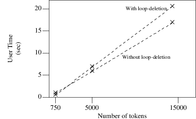
Time measurements on processing three C-programs with and without the loop-deletion algorithm

The diagram shows that the loop-deletion algorithm does not dramatically slow down the recognizing process. There is, however, a measurable time loss of ±25%. As we will see later, the loop-deletion algorithm will turn out to be extremely useful in efficient use of memory when there are many loops in the graph.

The effect of the loop-detecion algorithm on parsing Modula-2 programs is even less than with C-programs; in fact there is no measurable time loss:

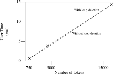
Time measurements on processing three Modula-2-programs with and without a loop-deletion algorithm

There are at least two reasons for this; both result from the relative simplicity of the Modula-2 grammar. The distance from a head to an end of stack marker is shorter than in C, and secondly Modula-2 causes fewer joins to occur than C, meaning that the loop marking algorithm is run less often and when it is run it has fewer paths to search.

3.1.4. Space measurements on the effect of leaving out theloop-deletion algorithm

Clearly, to make any measurements on the space-usage effects of leaving out the loop-deletion algorithm we need a program that causes the prediction graph to contain loops; however, we have not been able to devise a C or Modula-2 program that does this. In order to be able to make measurements, we added an extra alternative to a rule of the C compiler grammar, making it directly left-recursive. To make LLgen accept this new grammar, we put a ‘%if’ directive in the rule.

We have input our standard C test program consisting of 800 tokens to the error recovery routine for this ‘doctored’ C compiler, and compared the storage needed for the prediction graphs with the loop deletion algorithm enabled with the storage needed when the algorithm is disabled. With the loop-deletion algorithm enabled, the maximum size of the prediction graph was 5576 bytes. When the loop algorithm was disabled, the maximum size of the prediction graph grew to 12676 bytes; furthermore, 12676 bytes of heap were allocated for the prediction graph, but not deallocated again, because they were in use by graph elements that were in inaccessible loops. The user-time the program needed decreased only slightly, from 0.9 to 1.0 seconds. Given the relatively small input program, this data suggests that when loops are actually being made, the loop deletion algorithm is definitely worth the extra overhead it costs, considering the space that would otherwise be occupied by inaccessible loops. To verify this, we input the C program consisting of 15000 tokens to the compiler; execution time increased from 17.3 to 21.1 seconds after enabling the loop deletion algorithm, while the maximum size of the prediction graph shrunk from 328664 to 13664 bytes. With the loop-deletion algorithm disabled, 326720 bytes allocated for the graph were not deallocated again. Again, given the relatively small increase in execution time and the large reduction of memory usage, we feel that the loop-deletion algorithm is useful enough to justify the overhead it creates.

3.2. Problems encountered

In this section we describe some of the problems we encountered while testing the non-correcting error recovery.

3.2.1. The LLgen error reporting mechanism.

The parsers generated by LLgen call a user-supplied error reporting routine, usually called LLmessage. This routine is called with an integer parameter that is positive, zero or negative. When the parameter is positive the parser has just inserted a token, whose number is equal to the parameter; if it is zero, the parser has deleted a token whose number is in a global variable called LLsymb; if it is negative, it means that LLgen expected end-of-file, but did not find it. The routine LLmessage is supposed to print an error message, and when a token is inserted, it should set all necessary attributes.

However, when non-correcting error recovery is used, the situation becomes slightly different; when the parser inserts a token, it is only to keep the semantic actions consistent, and does no longer signify an error. However, the LLmessage routine still has to be called because the attributes of the inserted token need to be set. Therefore, when non-correcting error recovery is used, the LLmessage routine should not print an error message when the parameter is positive, or else it will print highly confusing error messages indeed. Furthermore, the LLmessage routine will usually print a message like ‘token ... deleted’ when it is called with parameter equal to zero; however, when the non-correcting error recovery is used, it is more appropriate to report something like ‘token ... illegal’, as the non-correcting error recovery does not delete tokens. Finally, when an unexpected end-of-file is encountered, LLgen normally just inserts the missing tokens and calls LLmessage with the parameter equal to the token number; when non-correcting error recovery is used we need a way to actually report we have encountered an unexpected end-of-file. The way we achieved this is by calling LLgen with parameter 0 and the global variable LLsymb set to EOFILE when this situation occurs; the routine LLmessage should print something like ‘unexpected end of file’ when it is called with parameter 0 and LLsymb is EOFILE. To facilitate switching between correcting and non-correcting error recovery, the file Lpars.h contains a statement ‘#define LLNONCORR’ if non-correcting error recovery is used.

3.2.2. Parsers being started in semantic actions

LLgen allows the programmer to define more than one nonterminal as the start symbol of the input grammar; it will generate a parsing routine for each of the start symbols. However, the error recovery code is generated only once; it is shared by all parsers. The programmer is free to call any of the generated parsers whenever he wants; for instance, in the C-compiler a separate parser for expressions in #if and #elsif statements is used. Whenever the lexical analyzer encounters such a statement, it calls the expression parser. It is also possible to call a parser in a semantic action of another parser; in the MODULA-2 compiler a separate parser for definition modules is used. When the main parser encounters a FROM defmod IMPORT statement a semantic actions opens the definition module defmod and starts the parser for definition modules.

The fact that subparsers can be started just about anywhere causes problems when non-correcting error recovery is used. Suppose a parser calls another parser in a semantic action to parse a separate input file. In the Modula-2 compiler, after seeing the FROM defmod IMPORT statement a semantic action opens defmod and parses it; now, if a syntax error occurred before the FROM IMPORT statement, the non-correcting error recovery will not execute the action that opens and parses the definition module, but it will not report an error either, because the statement FROM defmod IMPORT is part of the input language of the main parser. However, suppose that during the parsing of a definition module an error occurs; then, some semantic actions that would normally be executed during parsing of the definition module will not have taken place. When normal parsing is now resumed by the main parser, after the non-correcting error recovery has finished with the definition module, a lot of spurious semantic errors are likely to be reported, because the semantic actions that would normally have been executed during the definition module parsing have not been executed by the error recovery. Therefore, it is desirable that the main parser does not resume normal parsing, but instead continues with the non-correcting error recovery as well. Any syntactic errors in the main program will still be reported, but no spurious semantic errors will be reported that way.

When the lexical analyzer calls other parsers, as is the case in the ACK C compiler, recursive invocations of the non-correcting error recovery routine can occur. This will happen if a parser starts the error recovery, the error recovery calls the lexical analyzer, which starts another parser that finds a syntax error and calls the error recovery again. This is not really a problem, but is has consequences for the implementation of the error recovery routine.

The worst case occurs when two parsers are involved in parsing one input file, and the secondary parser (e.g. an inline assembly parser) is called in a semantic action of the main parser. Suppose now that the input text contains a syntax error; after detecting this error, the parser starts the non-correcting error recovery. This recovery does not execute any semantic actions; therefore it will not start the subparser at those points where the original LLgen generated parser would. As a result, parts of the program that would be accepted by the subparser will now probably be rejected as illegal, because the error recovery does not know it should use another grammar to check these parts. This is a serious problem, and we have devised and implemented two ways to solve it.

The first solution is based on the assumption that whenever a semantic action occurs in the grammar, another parser can be started at that point. Obviously, we have no way of knowing which semantic actions start a parser and which don’t, so we assume the worst. Now, assume that in the grammar there are k symbols defined as start symbols, say . Each of these symbols will cause LLgen to generate a parser that can be called in any of the semantic actions of the grammar. We now introduce a new symbol , and a new grammar rule . In the grammar the error recovery algorithm uses, we insert this symbol X at all positions where there are semantic actions in the original grammar, so a rule { action } becomes . As a result, at each position in a grammar rule where a semantic action occurs, we now accept any input that would be accepted by any of the parsers. Clearly, this solution is somewhat of a kludge, as it will accept a lot of input that is not accepted by the original parser. However, it is guaranteed to never give spurious error messages, because whenever a parser would be started by the original parser, there now is an in the grammar that produces all the strings that would be accepted by that parser. We have implemented this solution, and found it to be extremely slow, which of course was to be expected given the number of semantic actions in the average grammar. Furthermore, because each time a semantic action occurs in the grammar a string accepted by any of the generated parsers is accepted, including strings recognized by the currently running parser, error messages become hard to interpret. As an example, consider the following C program:

Clearly, there is a ‘)’ missing in the while-statement; however, if this program is input to the error recovery it will complain "} illegal", since after recognizing the expression controlling the while the original parser starts a semantic action, so the non-correcting recovery will accept a valid C program at that point; after recognizing the three statements following the while-statement as a separate program the recognizer expects the missing ‘)’, but gets ‘}’ instead.

Our second solution is based on the observation that if we knew which semantic actions can start other parsers, we would only have to introduce the new symbol at those places where parsers can get started. We have therefore extended LLgen with a new directive %substart, which is used to indicate to the parser generator that another parser may be started. The %substart is followed by the startsymbols that will produce the parsers that can be called, so %substart A, B, C; indicates that in the semantic action following the directive the parsers produced by startsymbols A, B, en C can be started. In the grammar used by the error recovery, a new symbol will be introduced at this point, along with a new rule . Of course, this solution can still accept input that would not have been accepted by original parser, for instance if a parser is started conditionally, based on other semantic information. However, it is a big improvement over the first solution, both in performance and the input it accepts.

3.2.3. Syntactic errors being handled in semantic actions

A programmer may decide to handle certain syntactic errors in semantic actions, for instance because he is not satisfied with the standard error recovery. However, since the non-correcting error recovery does not execute semantic actions, this may cause errors to remain undetected. We encountered the following example in the ACK Modula-2 compiler, in the grammar rule for assignment statement:

This works well in the original LLgen; however, statements like ‘j=9’ are not treated as syntactic, but as semantic errors. The original LLgen generated parser will print the (semantic) error message, but the non-correcting recovery will not execute the semantic action and therefore the erroneous input will be accepted.

To facilitate the incorporation of non-correcting error recovery in parsers that use this kind of ‘trick’, we extended LLgen with the %erroneous directive. The directive indicates to the non-correcting recovery mechanism that the token following it is not really part of the grammar. When recognizing input, the error recovery will ignore tokens in the grammar that have %erroneous in front of them. If in the example above, the ’=’ is replaced with %erroneous ’=’, the non-correcting mechanism will report an error when it sees a statement like ’j = 9’. See appendix B for details about the implementation of the %erroneous directive.

Another example is in the ACK C compiler. For some reason, the grammar accepts function definitions without ‘()’, so according to the syntax a function definition can look like:

The absence of the ‘()’, however, causes ‘func’ to be entered in the symbol table as non-function, and when the parser encounters the body a semantic action will complain with the error message "Making function body for non-function". This again will cause the non-correcting error recovery to miss errors. Consider this piece of code:

int i int j = 1;
{}

where apparently there’s a ‘;’ missing between the declarations of i and j. The original LLgen-generated parser only gives semantic errors:
"Making function body for non-function"
"j is not in parameter list"
"Illegal initialization of formal parameter, ignored"

As a result, the non-correcting error recovery will not report any errors in this piece of code, because it does not execute the semantic actions that recognize and report the error. Unfortunately, due to the way the C-grammar is written, it is not possible to solve this problem using a %erroneous directive; the part of the grammar that deals with declaratons would have to be rewritten so as to syntactically reject functions without ‘()’.

3.2.4. Semantic actions that read input

There are no restrictions on what a semantic action can do; there is nothing to stop the programmer from writing a parser in such a way that some of the input to the parser is processed by semantic actions. Obviously, because the non-correcting error recovery does not execute semantic actions, this kind of parser will not work at all with the new error recovery. Ironically, LLgen itself is written in such a fashion; {}-enclosed C-code in its input is processed by a semantic action in the LLgen grammar. We feel that it is bad practice to write parsers this way; the ‘eating’ of parts of the input should be done in the lexical analyzer, not in the parser. After all, in the case of LLgen, one can regard a semantic action in the input as one token, and thus it should be handled by the lexical analyzer as such.

3.3. Examples of error recovery

We will now give some examples that compare non-correcting error recovery with the correcting error recovery used by parsers generated by ‘standard’ LLgen.

Consider the next C program, where there is a ‘)’ missing in the header of function ‘test’.

This small error derails the ‘standard’ parser; it produces the following error messages, where we have left out 7 messages reporting semantic errors:

In contrast, the parser using non-correcting error recovery produces only one error message:

This error message correctly pin-points the error: there should have been a ‘)’ at the position where type-identifier ‘int’ is.

Now, an example with Modula-2; consider this program:

There are two syntactic errors in this program; on line 3, TYPES should be TYPE, and on line 10, VARS should be VAR. We have left out the type declarations of ElementType and ElementPointerType; clearly this will generate semantic errors, but we are only interested in syntactic errors anyway. The correcting error recovery parser again derails on this program; it produces the following syntactic error messages:

The error correction mechanism clearly makes the wrong guess by inserting CONST on line 3; as a result, all that follows is rejected as incorrect. In contrast, the non-correcting error recovery mechanism only produces two error messages:

This again exactly pin-points the errors: the identifiers TYPES and VARS constitute the only errors in the program. Note that the presence of more than one error does not cause any problems to the non-correcting recovery mechanism.

4. Conclusion

After implementing and testing a non-correcting error recovery mechanism we have come to the conclusion that it indeed is superior to correcting mechanisms in what regards the error messages it produces; the examples we have given clearly show this. However, there is a clear loss of performance when errors are present in a program, although we have found this performance degradation to be acceptable. We feel that the benefits of better error messages outweigh the loss of performance. In any case, correct programs do not suffer at all from the incorporation of a non-correcting recovery mechanism. The error recovery mechanism we implemented does not make unreasonable demands on resources; the size of the prediction graphs stays within reasonable limits.

The main problems we encountered had to do with recognizing ‘languages within languages’, and semantic actions that did unreasonable things like eating input. The more ‘well-behaved’ a parser is, the better the results the non-correcting error recovery mechanism gives. This is also true for the input grammars: with a language like Modula-2, whose syntax has been designed with parser generators in mind, the performance of the non-correcting mechanism is better than with C, whose syntax is extremely hard, if not impossible to describe with a LL(1) grammar.

5. Bibliography

Appendix A: Implementation Issues

In this appendix we will describe some implementation issues; the data structure used to store the grammar during non-correcting error recovery, postponing deletions of graph elements until after the prediction phase, and the implementation of the %substart directive .

A.1 The grammar data structure

The grammar data structure used by the non-correcting error recovery technique has to meet two conditions: easy access to a rule as a whole to make substituting nonterminals efficient and easy access to each symbol in the RHS of a rule to make starting error recovery and finding continuations efficient. To fulfill these conditions we decided to construct the storage of the grammar as follows.

A rule in the grammar is divided in two parts: a LHS and a RHS. The LHS is represented by a struct ‘lhs’ and for each symbol in the RHS a struct ’symbol’ is constructed. A struct ‘lhs’ contains the number of the nonterminal forming the LHS of the rule, a pointer to the RHS, the first- and follow-sets of the nonterminal and a flag ’empty’ which indicates whether the nonterminal produces empty or not. A struct ‘symbol’ contains a field indicating the type of the symbol, i.e. a terminal or a nonterminal, the number of the symbol, a ‘link’ pointer to a struct ‘symbol’ that represents the same symbol, a ‘next’ pointer to the rest of the RHS and a pointer back to the LHS.

A special struct ‘symbol’ is added to the end of the RHS to indicate the end of a rule. The type of this struct is LLEORULE, the number is set to -1 and the pointers ’link’ and ‘next’ are nil.

In case that there is more than one RHS for a LHS, all the RHS’s are put after each other and separated by another special struct ‘symbol’. The type of this struct is LLALT, the number is set to -1 and the ’link’ pointer is nil. After the last RHS a ‘LLEORULE’-struct marker is added.

Finally, to make searching efficient there are two arrays: ‘terminals’ and ‘nonterminals’. ‘terminals’ is indexed by the number of a terminal and contains for each terminal a struct containing a ’link’ pointer to a symbol, representing this terminal, in the RHS of a rule. Because this symbol has again a ’link’ pointer to another symbol representing the terminal, it is possible by following this chain of pointers to find all rules containing such a terminal. In a similar way ‘nonterminals’ is indexed by the number of a nonterminal and contains for each nonterminal a struct. This struct not only contains a ’link’ pointer linking all rules with this nonterminal, but also contains a ’rule’ pointer. This pointer points to the RHS or RHS’s of the rules of which the nonterminal forms the LHS.

As an example, consider the following grammar:

This will result in the picture below. Note that ‘pointer’ fields without an arrow indicate nil pointers.

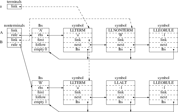
Note that the empty alternative for ‘B’ is represented in the data structure by the ‘LLEORULE-struct’ immediately following the ‘LLALT’-struct. When there are still other alternatives the ‘LLEORULE’-struct is replaced by a ‘LLALT’-struct followed by the other alternatives and a ‘LLEORULE’-struct. Finally, when the empty rule is the only rule for a nonterminal the RHS will consist only of a ‘LLEORULE’-struct.

A.2 Delayed deletes

We encountered a problem with deleting elements during the prediction phase. Imagine that we have a nonterminal ‘B’ on top of the graph, and ‘B’ has two alternatives. Now suppose that we apply the first alternative and we find out that this alternative leads to a ‘dead end’, i.e. a head that does not match the input symbol, so we want to get rid of it. When we delete it immediately the deletion algorithm will also deallocate ‘[B]’ and possibly some elements below ‘[B]’. However, there was another alternative for ‘[B]’ which was not yet developed and maybe this alternative leads to a head which is legal. But ‘[B]’ has already been deleted and thus cannot be used anymore. A similar situation can occur when we want to delete a joined element; the substitution of a nonterminal that only produces empty and thus has no element above it in the graph can also lead to such a situation. We therefore decided to put ‘dead ends’ on a list, ‘cleanup_arr[]’, and after the prediction phase has finished we delete all elements on this list, and all their descendants that become unreachable of course.

A.3 Clearing flags

We implemented two different ways to clear the flags set by the prediction phase of the algorithm; the first recursively tracks down the whole graph following the flags, the second puts all elements visited by the prediction phase on a list; after the prediction phase has finished the algorithm walks through this list clearing the flags of all elements on it. We took measurements on both algorithms and found out that with small programs the times did not differ much but large programs were processed faster by the second algorithm. Therefore we decided to use the second algorithm.

To speed up the algorithm even more, we do not deallocate the list after a prediction phase has finished. We just set the number of elements on the list to 0. This saves considerably on the number of ‘Malloc’-calls.

A.4 Implementation of %erroneous directive

As explained in chapter 3, the user can put a %erroneous directive in front of a terminal, making the non-correcting error recovery mechanism ignore that terminal. However, implementing this directive was not entirely straightforward; consider, for example, the rule

Just leaving out terminal ’b’ will not do, because then nonterminal A produces empty all of a sudden, which it did not before. The rule should become

but this is hard to implement in LLgen. We took a different approach: we introduce a new terminal ’ERRONEOUS’, and substitute it for all terminals with an %erroneous directive in front of them. Thus, the example rule becomes

Since the terminal ERRONEOUS will never be in the input to the parser, this has exactly the desired effect; when a predicting phase produces ERRONEOUS as head of a prediction graph this head will never match the input. In particular, it will not match the terminal that was originally there (in this case ’b’) so that terminal is no longer regarded as part of the input language at that point.

Appendix B: Using the non-correcting error recovery

To use the new non-correcting error recovery mechanism, LLgen has to be called with the new flag -n. LLgen will then create an extra file called ‘Lncor.c’ which contains the code for the non-correcting recovery mechanism. This file has to be compiled and linked with the rest of the program, just like the file ‘Lpars.c’.

The user-supplied error reporting routine ‘LLmessage’ will have to be modified slightly; when it is called with a positive parameter, it should only set the attributes of the inserted token, but not report an error. Note that the lexical analyzer still must return the same token as it did the last time it was called. When LLmessage is called with parameter 0, it should report that the token in global variable LLsymb is illegal; if the value of LLsymb is ‘EOFILE’, the routine should report an unexpected End-of-file. When LLmessage is called with parameter -1, it should report that end-of-file was expected. To facilitate switching between correcting and non-correcting error recovery, the file Lpars.h contains a statement ‘#define LLNONCORR’ which indicates that the non-correcting mechanism is enabled. Here is a skeleton for the modified LLmessage routine:

#ifndef LLNONCORR

#endif

#ifndef LLNONCORR

#else

#endif

For best results, one should check if the parser calls other parsers in semantic actions; if this is the case, and the called parser processes the same input file as the calling parser, then a %substart should be put in front of the semantic action that starts a parser. If a semantic action calls parsers defined by startsymbols say A and B, then ‘%substart A, B;’ should be put in front of the action. As an alternative, one can use the -s flag of LLgen; this has the same effect as putting ‘%substart X, Y, ....;’ in front of all semantic actions, where X, Y, .... are the startsymbols of the grammar. Clearly, it is preferable to analyze the grammar and put %substart directives only where appropriate.

Finally, beware of syntactic errors being handled in semantic actions; eg, one could have a rule like

Assignment_statement: lvalue
[
’=’
{
error(":= expected");
}

|

’:=’
]
expression
;

To ensure that the non-correcting mechanism will recognize the ‘=’ as a syntactic error, a ‘%erroneous’ directive should be put in front of it.